Bootstrapping
October 7 + 9 + 16, 2024
Agenda 10/7/24
- Review: logic of SE
- Logic of bootstrapping (resample from the sample with replacement)
- BS SE of a statistic
Why bootstrap?
Motivation:
to estimate the variability and distribution of a statistic in repeated samples of size
(not dependent on being true).
Variability
standard deviation of the data:
standard error of the statistic: depends…
Intuitive understanding
See in the applets for an intuitive understanding of both confidence intervals and boostrapping:
StatKey applets which demonstrate bootstrapping.
Confidence interval logic from the Rossman & Chance applets.
Basic Notation
(n.b., we don’t ever do what is on this slide)
Let
Ideally
(we never do part (a))
Bootstrap Procedure
- Resample data with replacement from the original sample.
- Calculate the statistic of interest for each resample.
- Repeat 1. and 2.
- Use the bootstrap distribution for inference.
Bootstrap Notation
(n.b., bootstrapping is the process on this slide)
Take many (
Let
What do we get?
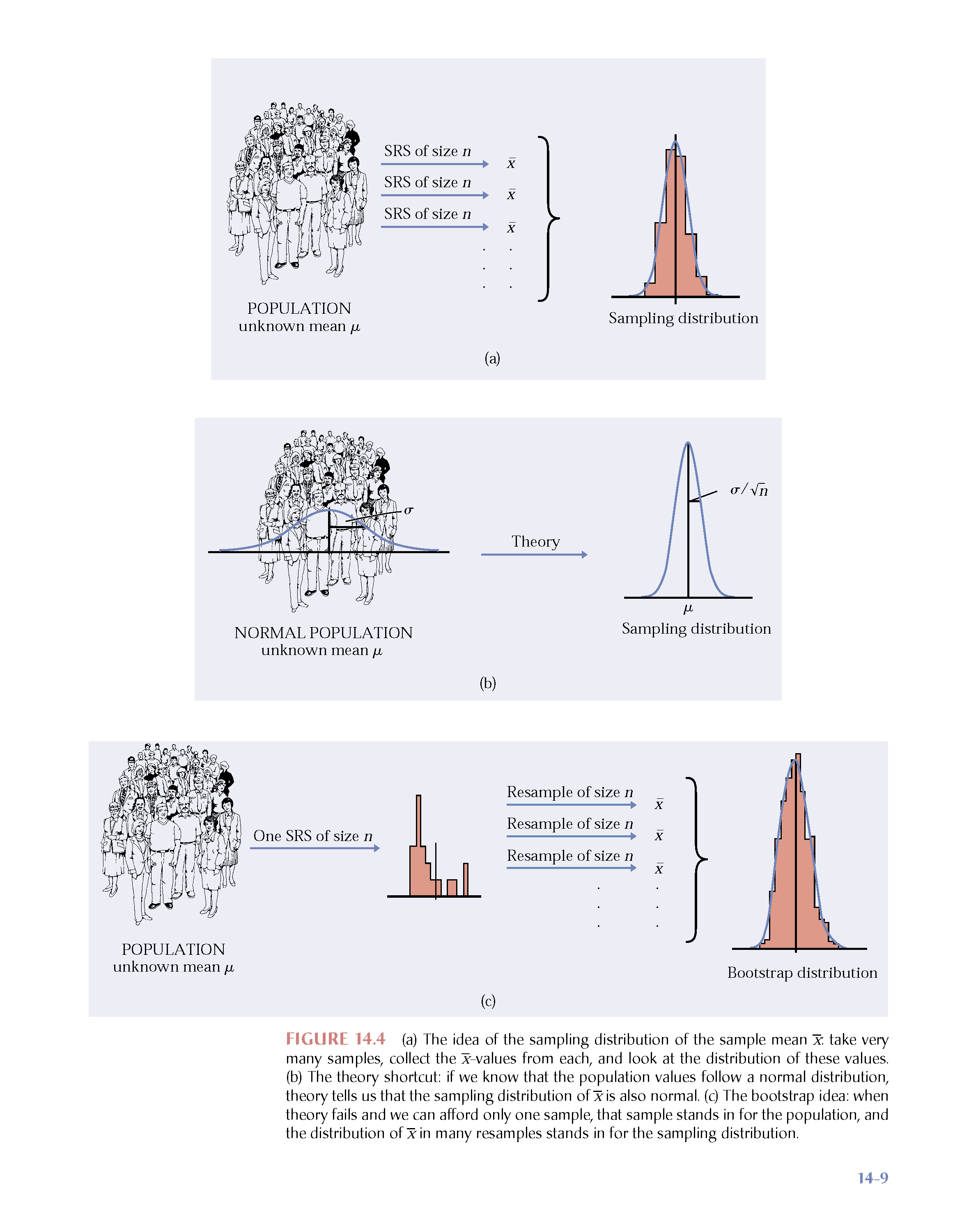
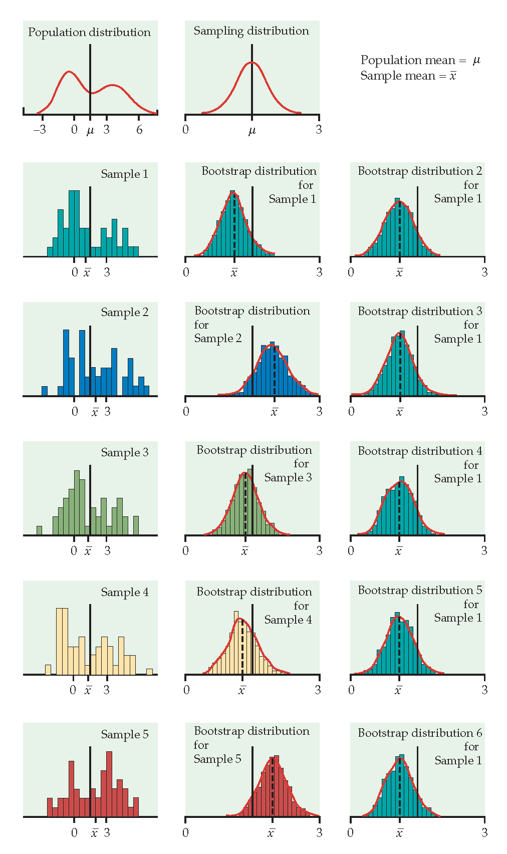
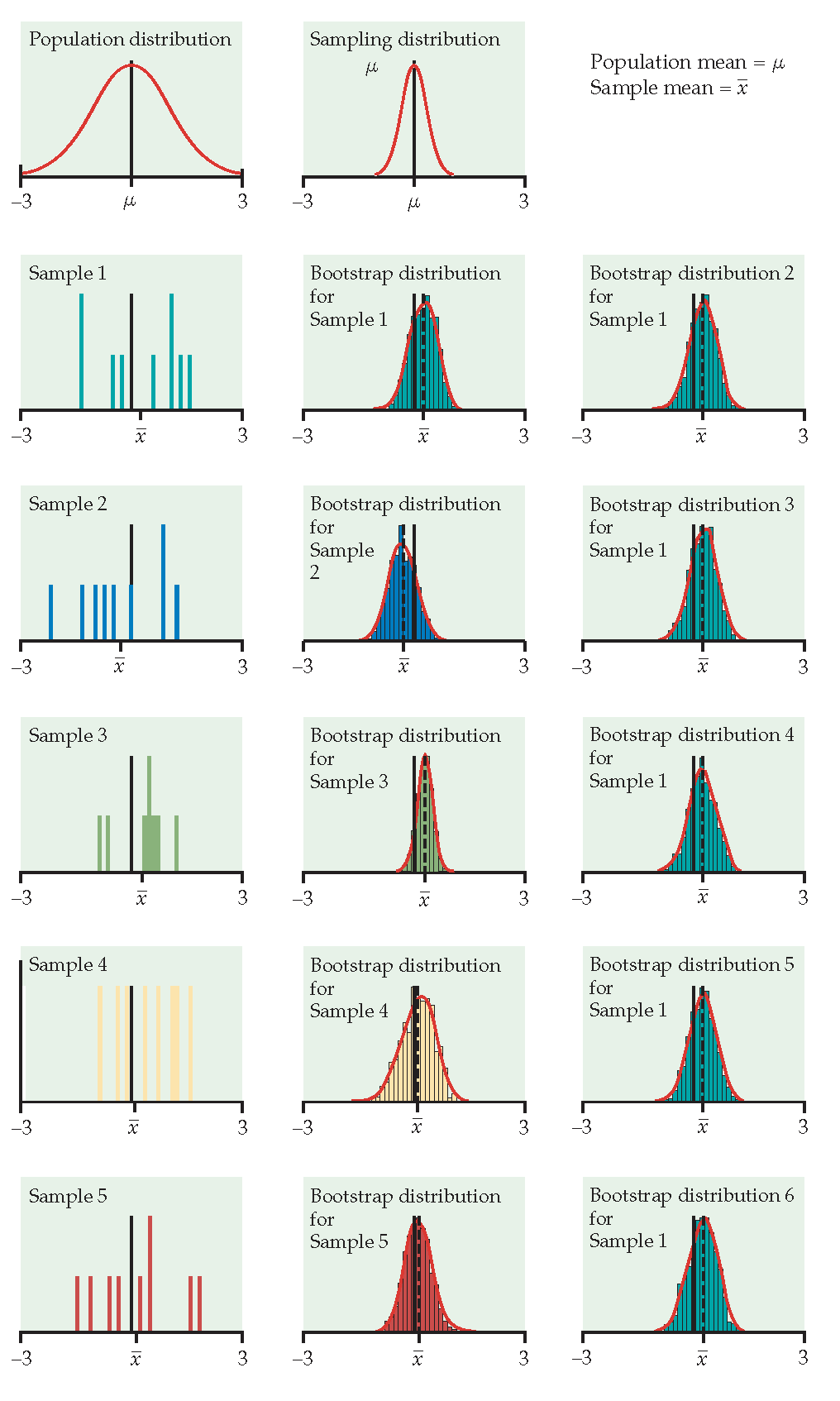
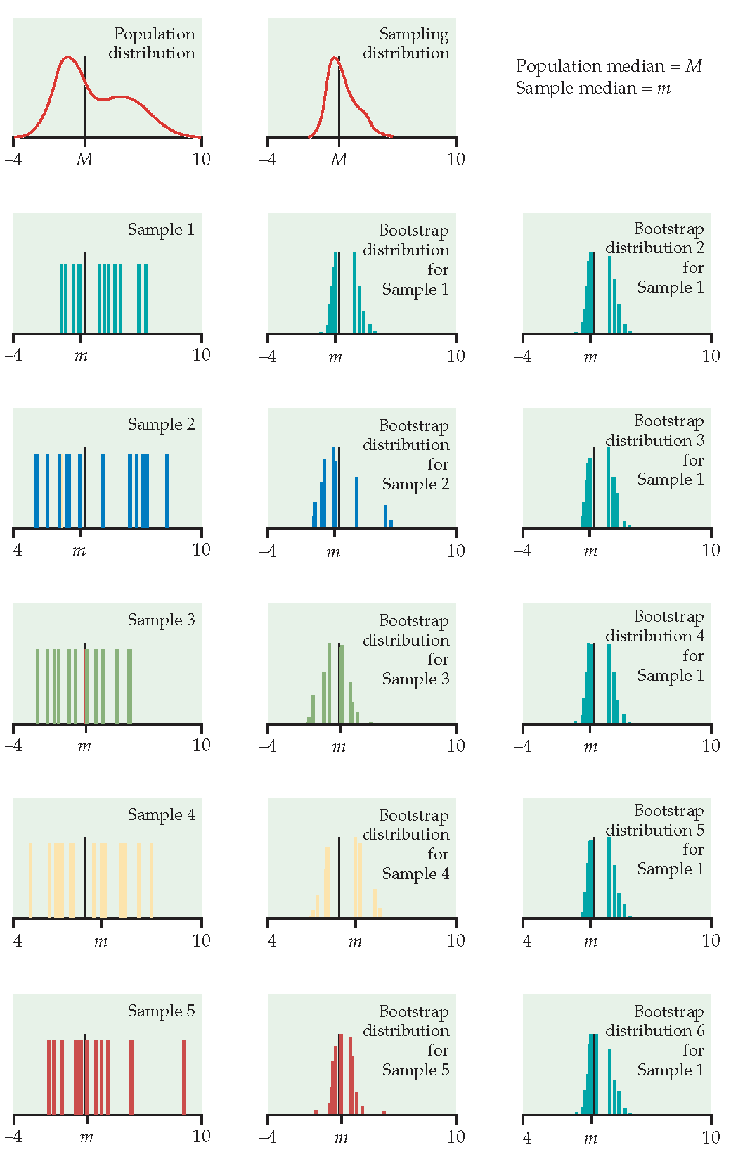
Just like repeatedly taking samples from the population, taking resamples from the sample allows us to characterize the bootstrap distribution which approximates the sampling distribution.
The bootstrap distribution approximates the shape, spread, & bias of the true sampling distribution.
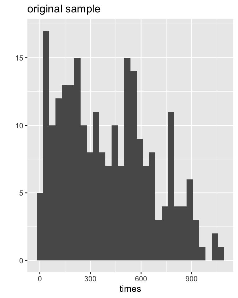
Example
Everitt and Rabe-Hesketh (2006) report on a study by Caplehorn and Bell (1991) that investigated the time (days) spent in a clinic for methadone maintenance treatment for people addicted to heroin.
The data include the amount of time that the subjects stayed in the facility until treatment was terminated.
For about 37% of the subjects, the study ended while they were still the in clinic (status=0).
Their survival time has been truncated. For this reason we might not want to estimate the mean survival time, but rather some other measure of typical survival time. Below we explore using the median as well as the 25% trimmed mean. (From Chance and Rossman (2018), Investigation 4.5.3)
The data
# A tibble: 238 × 5
      id clinic status times  dose
   <dbl>  <dbl>  <dbl> <dbl> <dbl>
 1     1      1      1   428    50
 2     2      1      1   275    55
 3     3      1      1   262    55
 4     4      1      1   183    30
 5     5      1      1   259    65
 6     6      1      1   714    55
 7     7      1      1   438    65
 8     8      1      0   796    60
 9     9      1      1   892    50
10    10      1      1   393    65
# ℹ 228 more rows
Observed Test Statistic(s)
heroin |>
  summarize(obs_med = median(times),
            obs_tr_mean = mean(times, trim = 0.25))
# A tibble: 1 × 2
obs_med obs_tr_mean
<dbl> <dbl>
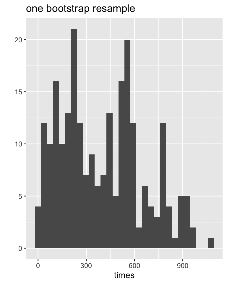
1 368. 378.Bootstrapped data!
set.seed(4747)

heroin |>
  sample_frac(size=1, replace=TRUE) |>
  summarize(boot_med = median(times),
            boot_tr_mean = mean(times, trim = 0.25))
# A tibble: 1 × 2
boot_med boot_tr_mean
<dbl> <dbl>
1 368 372.Bootstrapping with map().
n_rep1 <- 100
n_rep2 <- 20
set.seed(4747)heroin# A tibble: 238 × 6
id clinic status times prison dose
<dbl> <dbl> <dbl> <dbl> <dbl> <dbl>
1 1 1 1 428 0 50
2 2 1 1 275 1 55
3 3 1 1 262 0 55
4 4 1 1 183 0 30
5 5 1 1 259 1 65
6 6 1 1 714 0 55
7 7 1 1 438 1 65
8 8 1 0 796 1 60
9 9 1 1 892 0 50
10 10 1 1 393 1 65
# ℹ 228 more rowsboot_stat_func <- function(df){
df |>
mutate(obs_med = median(times),
obs_tr_mean = mean(times, trim = 0.25)) |>
sample_frac(size=1, replace=TRUE) |>
summarize(boot_med = median(times),
boot_tr_mean = mean(times, trim = 0.25),
obs_med = mean(obs_med),
obs_tr_mean = mean(obs_tr_mean))}boot_1_func <- function(df){
df |>
sample_frac(size=1, replace=TRUE)
}map(1:n_rep1, ~boot_stat_func(df = heroin)) |>
list_rbind()# A tibble: 100 × 4
boot_med boot_tr_mean obs_med obs_tr_mean
<dbl> <dbl> <dbl> <dbl>
1 368 372. 368. 378.
2 358 363. 368. 378.
3 431 421. 368. 378.
4 332. 350. 368. 378.
5 310. 331. 368. 378.
6 376 382. 368. 378.
7 366 365. 368. 378.
8 378. 382. 368. 378.
9 394 386. 368. 378.
10 392. 402. 368. 378.
# ℹ 90 more rowsData distributions
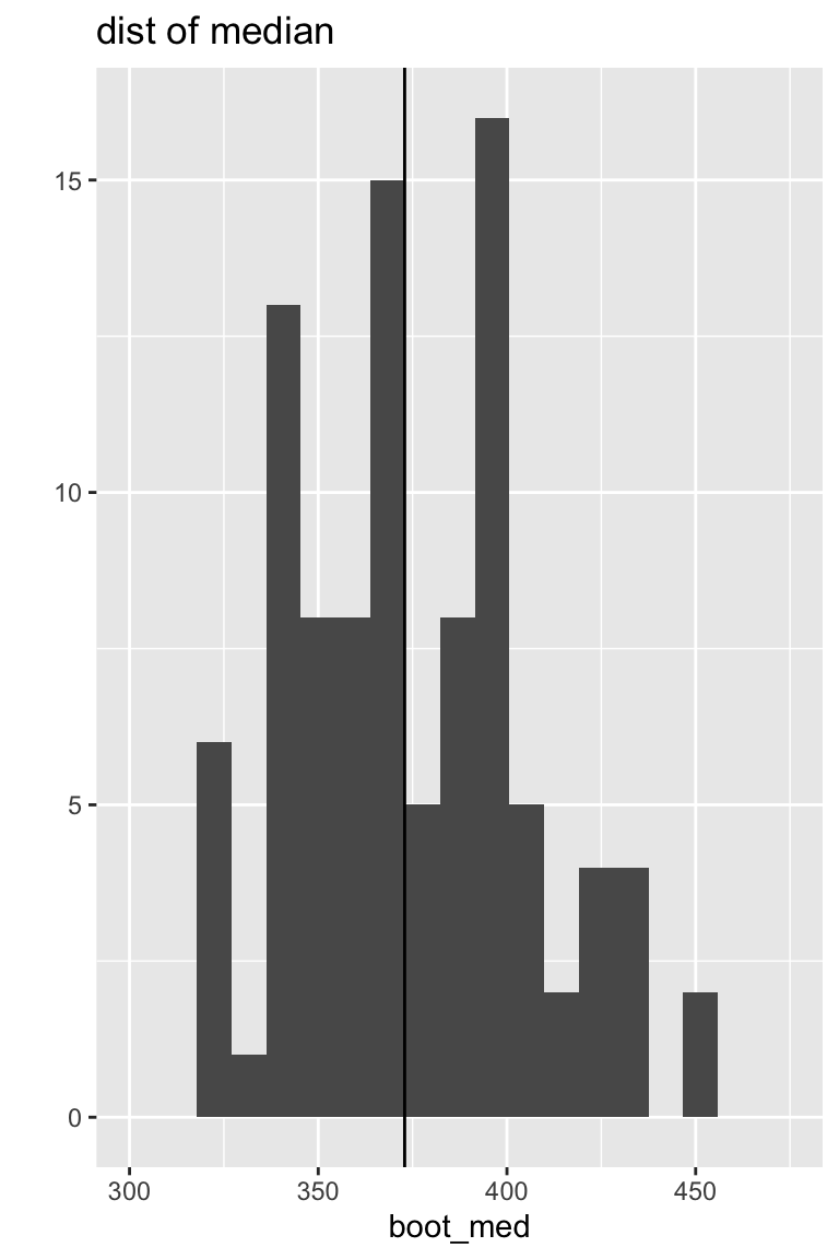
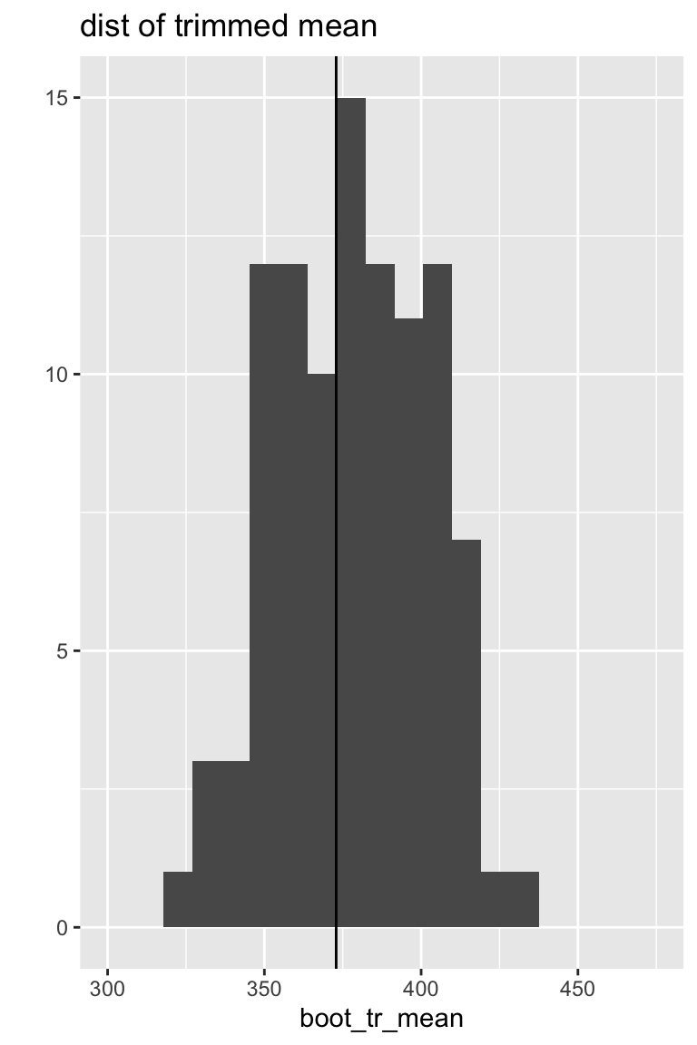
Sampling distributions
Both the median and the trimmed mean are reasonably symmetric and bell-shaped.
Agenda 10/16/24
- Logic of CI
- Normal CI using BS SE
- Bootstrap-t (studentized) CIs
- Percentile CIs
- properties / advantages / disadvantages
Technical derivations
See in class notes on bootstrapping for the technical details on how to create different bootstrap intervals.
Bootstrapping with map
n_rep1 <- 100
set.seed(4747)
boot_stat_func <- function(df){
df |>
mutate(obs_med = median(times),
obs_tr_mean = mean(times, trim = 0.25)) |>
sample_frac(size=1, replace=TRUE) |>
summarize(boot_med = median(times),
boot_tr_mean = mean(times, trim = 0.25),
obs_med = mean(obs_med),
obs_tr_mean = mean(obs_tr_mean))}boot_stats <- map(1:n_rep1, ~boot_stat_func(df = heroin)) |>
list_rbind()
boot_stats# A tibble: 100 × 4
boot_med boot_tr_mean obs_med obs_tr_mean
<dbl> <dbl> <dbl> <dbl>
1 368 372. 368. 378.
2 358 363. 368. 378.
3 431 421. 368. 378.
4 332. 350. 368. 378.
5 310. 331. 368. 378.
6 376 382. 368. 378.
7 366 365. 368. 378.
8 378. 382. 368. 378.
9 394 386. 368. 378.
10 392. 402. 368. 378.
# ℹ 90 more rows95% normal CI with BS SE
boot_stats |>
  summarize(
    low_med = mean(obs_med) + qnorm(0.025) * sd(boot_med),
    up_med = mean(obs_med) + qnorm(0.975) * sd(boot_med),
    low_tr_mean = mean(obs_tr_mean) + qnorm(0.025) * sd(boot_tr_mean),
    up_tr_mean = mean(obs_tr_mean) + qnorm(0.975) * sd(boot_tr_mean))
# A tibble: 1 × 4
low_med up_med low_tr_mean up_tr_mean
<dbl> <dbl> <dbl> <dbl>
1 310. 425. 337. 420.95% Percentile CI
boot_stats |>
  summarize(perc_CI_med = quantile(boot_med, c(0.025, 0.975)),
            perc_CI_tr_mean = quantile(boot_tr_mean, c(0.025, 0.975)),
            q = c(0.025, 0.975))
# A tibble: 2 × 3
perc_CI_med perc_CI_tr_mean q
<dbl> <dbl> <dbl>
1 321 335. 0.025
2 435. 420. 0.975Double bootstrapping with map
n_rep1 <- 100
n_rep2 <- 20
set.seed(4747)
boot_stat_func <- function(df){
df |>
mutate(obs_med = median(times),
obs_tr_mean = mean(times, trim = 0.25)) |>
sample_frac(size=1, replace=TRUE) |>
summarize(boot_med = median(times),
boot_tr_mean = mean(times, trim = 0.25),
obs_med = mean(obs_med),
obs_tr_mean = mean(obs_tr_mean))}boot_1_func <- function(df){
df |>
sample_frac(size=1, replace=TRUE)
}boot_2_func <- function(df, reps){
resample2 <- 1:reps
df |>
summarize(boot_med = median(times), boot_tr_mean = mean(times, trim = 0.25)) |>
cbind(resample2, map(resample2, ~df |>
sample_frac(size=1, replace=TRUE) |>
summarize(boot_2_med = median(times),
boot_2_tr_mean = mean(times, trim = 0.25))) |>
list_rbind()) |>
select(resample2, everything())
}boot_2_stats <- data.frame(resample1 = 1:n_rep1) |>
mutate(first_boot = map(1:n_rep1, ~boot_1_func(df = heroin))) |>
mutate(second_boot = map(first_boot, boot_2_func, reps = n_rep2)) Summarizing the double bootstrap
boot_2_stats |>
  unnest(second_boot) |>
  unnest(first_boot)
# A tibble: 476,000 × 12
resample1 id clinic status times prison dose resample2 boot_med
<int> <dbl> <dbl> <dbl> <dbl> <dbl> <dbl> <int> <dbl>
1 1 257 1 1 204 0 50 1 368
2 1 230 1 0 28 0 50 1 368
3 1 229 1 1 216 0 50 1 368
4 1 186 2 0 683 0 100 1 368
5 1 119 2 0 684 0 65 1 368
6 1 73 1 0 405 0 80 1 368
7 1 41 1 1 550 1 60 1 368
8 1 75 1 0 905 0 80 1 368
9 1 68 1 0 439 0 80 1 368
10 1 224 1 1 546 1 50 1 368
# ℹ 475,990 more rows
# ℹ 3 more variables: boot_tr_mean <dbl>, boot_2_med <dbl>,
# boot_2_tr_mean <dbl>boot_2_stats |>
unnest(second_boot) |>
unnest(first_boot) |>
filter(resample1 == 1) # A tibble: 4 × 4
skim_variable numeric.mean numeric.sd numeric.p50
<chr> <dbl> <dbl> <dbl>
1 boot_med 368 0 368
2 boot_tr_mean 372. 0 372.
3 boot_2_med 365. 32.5 367.
4 boot_2_tr_mean 368. 21.5 367.boot_t_stats <- boot_2_stats |>
unnest(second_boot) |>
unnest(first_boot) |>
group_by(resample1) |>
summarize(boot_sd_med = sd(boot_2_med),
boot_sd_tr_mean = sd(boot_2_tr_mean),
boot_med = mean(boot_med), # doesn't do anything, just copies over
boot_tr_mean = mean(boot_tr_mean)) |> # the variables into the output
mutate(boot_t_med = (boot_med - mean(boot_med)) / boot_sd_med,
boot_t_tr_mean = (boot_tr_mean - mean(boot_tr_mean)) / boot_sd_tr_mean)
boot_t_stats# A tibble: 100 × 7
resample1 boot_sd_med boot_sd_tr_mean boot_med boot_tr_mean boot_t_med
<int> <dbl> <dbl> <dbl> <dbl> <dbl>
1 1 32.5 21.5 368 372. -0.154
2 2 24.2 18.8 358 363. -0.619
3 3 32.0 21.1 431 421. 1.81
4 4 49.1 34.0 332. 350. -0.845
5 5 22.7 13.4 310. 331. -2.75
6 6 20.3 19.9 376 382. 0.148
7 7 35.3 22.1 366 365. -0.198
8 8 15.0 16.4 378. 382. 0.367
9 9 27.6 20.9 394 386. 0.761
10 10 38.5 19.6 392. 402. 0.481
# ℹ 90 more rows
# ℹ 1 more variable: boot_t_tr_mean <dbl>95% Bootstrap-t CI
Note that the t-value is needed (which requires a different SE for each bootstrap sample).
boot_t_stats |>
  select(boot_t_med, boot_t_tr_mean)
# A tibble: 100 × 2
boot_t_med boot_t_tr_mean
<dbl> <dbl>
1 -0.154 -0.249
2 -0.619 -0.790
3 1.81 2.04
4 -0.845 -0.824
5 -2.75 -3.50
6 0.148 0.235
7 -0.198 -0.570
8 0.367 0.261
9 0.761 0.406
10 0.481 1.26
# ℹ 90 more rowsboot_q <- boot_t_stats |>
select(boot_t_med, boot_t_tr_mean) |>
summarize(q_t_med = quantile(boot_t_med, c(0.025, 0.975)),
q_t_tr_mean = quantile(boot_t_tr_mean, c(0.025, 0.975)),
q = c(0.025, 0.975))
boot_q# A tibble: 2 × 3
q_t_med q_t_tr_mean q
<dbl> <dbl> <dbl>
1 -2.17 -2.20 0.025
2 1.78 2.06 0.975boot_q_med <- boot_q |> select(q_t_med) |> pull()
boot_q_med 2.5% 97.5%
-2.170931 1.782708 boot_q_tr_mean <- boot_q |> select(q_t_tr_mean) |> pull()
boot_q_tr_mean 2.5% 97.5%
-2.204115 2.059893 boot_t_stats |>
summarize(boot_t_CI_med = mean(boot_med) + boot_q_med*sd(boot_med),
boot_t_CI_tr_mean = mean(boot_tr_mean) + boot_q_tr_mean * sd(boot_tr_mean),
q = c(0.025, 0.975))# A tibble: 2 × 3
boot_t_CI_med boot_t_CI_tr_mean q
<dbl> <dbl> <dbl>
1 309. 331. 0.025
2 425. 421. 0.975Comparison of intervals
The first three columns correspond to the CIs for the true median of the survival times. The second three columns correspond to the CIs for the true trimmed mean of the survival times.
| CI | Lower | Obs Med | Upper | Lower | Obs Tr Mean | Upper |
|---|---|---|---|---|---|---|
| Percentile | 321 | 367.50 | 434.58 | 334.86 | 378.30 | 419.77 |
| w BS SE | 309.99 | 367.50 | 425.01 | 336.87 | 378.30 | 419.73 |
| BS-t | 309.30 | 367.50 | 425.31 | 331.03 | 378.30 | 421.17 |
(Can’t know what the Truth is…)
What makes a confidence interval procedure good?
That it captures the true parameter in
That it produces narrow intervals.
What else about intervals?
| CI | Symmetric | Range Resp | Trans Resp | Accuracy | Normal Samp Dist? | Other |
|---|---|---|---|---|---|---|
| Boot SE | Yes | No | No | 1st order | Yes | Parametric assumptions, |
| Boot-t | No | No | No | 2nd order | Yes/No | Computationally intensive |
| perc | No | Yes | Yes | 1st order | No | Small |
| BCa | No | Yes | Yes | 2nd order | No | Limited parametric assumptions |
References
:::
References
Caplehorn, JR, and J Bell. 1991. “Methadone Dosage and Retention of Patients in Maintenance Treatment.” The Medical Journal of Australia 154 (3): 195–99.
Chance, Beth, and Allan Rossman. 2018. Investigating Statistics, Concepts, Applications, and Methods. 3rd ed. http://www.rossmanchance.com/iscam3/.
Everitt, Brian S., and Sophia Rabe-Hesketh. 2006. Handbook of Statistical Analyses Using Stata. Chapman & Hall.