Computational Statistics – Support Vector Machines

What if the boundary is wiggly?

If a wiggly boundary is really best, and the value of $γ$ should be high to represent the high model complexity.

What if the boundary isn’t wiggly?

But if the boundary has low complexity, then the best value of $γ$ is probably much lower.

Simple decision boundary – gamma too big

Examples of kernels

linear $K (x, y) = x \cdot y$ Note, the only tuning parameter is the penalty/cost parameter $C$ ).
polynomial $K_{P} (x, y) = (γ x \cdot y + r)^{d} = ϕ_{P} (x) \cdot ϕ_{P} (y) γ > 0$ Note, here $γ, r, d$ must be tuned using cross validation (along with the penalty/cost parameter $C$ ).
RBF $K_{R B F} (x, y) = e^{(- γ | | x - y | |^{2})} = ϕ_{R B F} (x) \cdot ϕ_{R B F} (y)$ Note, here $γ$ must be tuned using cross validation (along with the penalty/cost parameter $C$ ).
sigmoid¹ $K_{S} (x, y) = \tanh (γ x \cdot y + r) = ϕ_{S} (x) \cdot ϕ_{S} (y)$ Note, here $γ, r$ must be tuned using cross validation (along with the penalty/cost parameter $C$ ). One benefit of the sigmoid kernel is that it has equivalence to a two-layer perceptron neural network.

Big $C$ or small $C$ ?

The low C value gives a large margin. On the right, the high C value gives a small margin. Which classifier is better? Well, it depends on what the actual data (test, population, etc.) look like! photo credit: http://stats.stackexchange.com/questions/31066/what-is-the-influence-of-c-in-svms-with-linear-kernel

Big $C$ or small $C$ ?

Now, the large C classifier is better. photo credit: http://stats.stackexchange.com/questions/31066/what-is-the-influence-of-c-in-svms-with-linear-kernel

Big $C$ or small $C$ ?

Now, the small C classifier is better. photo credit: http://stats.stackexchange.com/questions/31066/what-is-the-influence-of-c-in-svms-with-linear-kernel

Algorithm: Support Vector Machine

Using cross validation, find values of $C, γ, d, r$ , etc. (and the kernel function!)
Using Lagrange multipliers (read: the computer), solve for $α_{i}$ and $b$ .
Classify an unknown observation ( $u$ ) as “positive” if: $\sum α_{i} y_{i} ϕ (x_{i}) \cdot ϕ (u) + b = \sum α_{i} y_{i} K (x_{i}, u) + b \geq 0$

SVM example w defaults

penguin_svm_recipe <-
  recipe(sex ~ bill_length_mm + bill_depth_mm + flipper_length_mm +
           body_mass_g, data = penguin_train) |>
  step_normalize(all_predictors())

penguin_svm_recipe

── Recipe ──────────────────────────────────────────────────────────────────────

── Inputs

Number of variables by role

outcome:   1
predictor: 4

── Operations

• Centering and scaling for: all_predictors()

penguin_svm_lin <- svm_linear() |>
  set_engine("LiblineaR") |>
  set_mode("classification")

penguin_svm_lin

Linear Support Vector Machine Model Specification (classification)

Computational engine: LiblineaR

penguin_svm_lin_wflow <- workflow() |>
  add_model(penguin_svm_lin) |>
  add_recipe(penguin_svm_recipe)

penguin_svm_lin_wflow

══ Workflow ════════════════════════════════════════════════════════════════════
Preprocessor: Recipe
Model: svm_linear()

── Preprocessor ────────────────────────────────────────────────────────────────
1 Recipe Step

• step_normalize()

── Model ───────────────────────────────────────────────────────────────────────
Linear Support Vector Machine Model Specification (classification)

Computational engine: LiblineaR

penguin_svm_lin_fit <- 
  penguin_svm_lin_wflow |>
  fit(data = penguin_train)

penguin_svm_lin_fit

══ Workflow [trained] ══════════════════════════════════════════════════════════
Preprocessor: Recipe
Model: svm_linear()

── Preprocessor ────────────────────────────────────────────────────────────────
1 Recipe Step

• step_normalize()

── Model ───────────────────────────────────────────────────────────────────────
$TypeDetail
[1] "L2-regularized L2-loss support vector classification dual (L2R_L2LOSS_SVC_DUAL)"

$Type
[1] 1

$W
     bill_length_mm bill_depth_mm flipper_length_mm body_mass_g       Bias
[1,]       0.248908      1.080195        -0.2256375    1.328448 0.06992734

$Bias
[1] 1

$ClassNames
[1] male   female
Levels: female male

$NbClass
[1] 2

attr(,"class")
[1] "LiblineaR"

Fit again

══ Workflow [trained] ══════════════════════════════════════════════════════════
Preprocessor: Recipe
Model: svm_linear()

── Preprocessor ────────────────────────────────────────────────────────────────
1 Recipe Step

• step_normalize()

── Model ───────────────────────────────────────────────────────────────────────
$TypeDetail
[1] "L2-regularized L2-loss support vector classification dual (L2R_L2LOSS_SVC_DUAL)"

$Type
[1] 1

$W
     bill_length_mm bill_depth_mm flipper_length_mm body_mass_g       Bias
[1,]       0.248908      1.080195        -0.2256375    1.328448 0.06992734

$Bias
[1] 1

$ClassNames
[1] male   female
Levels: female male

$NbClass
[1] 2

attr(,"class")
[1] "LiblineaR"

SVM example w CV tuning (RBF kernel)

penguin_svm_recipe <-
  recipe(sex ~ bill_length_mm + bill_depth_mm + flipper_length_mm +
           body_mass_g, data = penguin_train) |>
  step_normalize(all_predictors())

penguin_svm_recipe

── Recipe ──────────────────────────────────────────────────────────────────────

── Inputs

Number of variables by role

outcome:   1
predictor: 4

── Operations

• Centering and scaling for: all_predictors()

penguin_svm_rbf <- svm_rbf(cost = tune(),
                           rbf_sigma = tune()) |>
  set_engine("kernlab") |>
  set_mode("classification")

penguin_svm_rbf

Radial Basis Function Support Vector Machine Model Specification (classification)

Main Arguments:
  cost = tune()
  rbf_sigma = tune()

Computational engine: kernlab

penguin_svm_rbf_wflow <- workflow() |>
  add_model(penguin_svm_rbf) |>
  add_recipe(penguin_svm_recipe)

penguin_svm_rbf_wflow

══ Workflow ════════════════════════════════════════════════════════════════════
Preprocessor: Recipe
Model: svm_rbf()

── Preprocessor ────────────────────────────────────────────────────────────────
1 Recipe Step

• step_normalize()

── Model ───────────────────────────────────────────────────────────────────────
Radial Basis Function Support Vector Machine Model Specification (classification)

Main Arguments:
  cost = tune()
  rbf_sigma = tune()

Computational engine: kernlab

set.seed(234)
penguin_folds <- vfold_cv(penguin_train,
                          v = 4)

# the tuned parameters also have default values you can use
penguin_grid <- grid_regular(cost(),
                             rbf_sigma(),
                             levels = 8)

penguin_grid

# A tibble: 64 × 2
        cost     rbf_sigma
       <dbl>         <dbl>
 1  0.000977 0.0000000001 
 2  0.00431  0.0000000001 
 3  0.0190   0.0000000001 
 4  0.0841   0.0000000001 
 5  0.371    0.0000000001 
 6  1.64     0.0000000001 
 7  7.25     0.0000000001 
 8 32        0.0000000001 
 9  0.000977 0.00000000268
10  0.00431  0.00000000268
# ℹ 54 more rows

# this takes a few minutes
penguin_svm_rbf_tune <- 
  penguin_svm_rbf_wflow |>
  tune_grid(resamples = penguin_folds,
            grid = penguin_grid)

penguin_svm_rbf_tune

# Tuning results
# 4-fold cross-validation 
# A tibble: 4 × 4
  splits           id    .metrics           .notes          
  <list>           <chr> <list>             <list>          
1 <split [186/63]> Fold1 <tibble [192 × 6]> <tibble [0 × 3]>
2 <split [187/62]> Fold2 <tibble [192 × 6]> <tibble [0 × 3]>
3 <split [187/62]> Fold3 <tibble [192 × 6]> <tibble [0 × 3]>
4 <split [187/62]> Fold4 <tibble [192 × 6]> <tibble [0 × 3]>

SVM model output

penguin_svm_rbf_tune |>
  collect_metrics() |>
  filter(.metric == "accuracy") |>
  ggplot() + 
  geom_line(aes(color = as.factor(cost), y = mean, x = rbf_sigma)) +
  geom_point(aes(color = as.factor(cost), y = mean, x = rbf_sigma)) +
  labs(color = "Cost") +
  scale_x_continuous(trans='log10')

SVM model output - take two

penguin_svm_rbf_tune |>
  collect_metrics() |>
  filter(.metric == "accuracy") |>
  ggplot() + 
  geom_line(aes(color = as.factor(rbf_sigma), y = mean, x = cost)) +
  geom_point(aes(color = as.factor(rbf_sigma), y = mean, x = cost)) +
  labs(color = "Cost") +
  scale_x_continuous(trans='log10')

SVM model output - best CV parameters

penguin_svm_rbf_tune |>
  collect_metrics() |>
  filter(.metric == "accuracy") |> 
  arrange(desc(mean))

# A tibble: 64 × 8
     cost rbf_sigma .metric  .estimator  mean     n std_err .config             
    <dbl>     <dbl> <chr>    <chr>      <dbl> <int>   <dbl> <chr>               
 1  0.371   1       accuracy binary     0.891     4 0.0123  Preprocessor1_Model…
 2 32       0.00139 accuracy binary     0.884     4 0.00747 Preprocessor1_Model…
 3  1.64    0.0373  accuracy binary     0.884     4 0.00747 Preprocessor1_Model…
 4 32       1       accuracy binary     0.880     4 0.0207  Preprocessor1_Model…
 5  1.64    1       accuracy binary     0.880     4 0.00791 Preprocessor1_Model…
 6  7.25    1       accuracy binary     0.872     4 0.0168  Preprocessor1_Model…
 7  7.25    0.0373  accuracy binary     0.872     4 0.0145  Preprocessor1_Model…
 8  7.25    0.00139 accuracy binary     0.868     4 0.0329  Preprocessor1_Model…
 9 32       0.0373  accuracy binary     0.868     4 0.0136  Preprocessor1_Model…
10  0.371   0.0373  accuracy binary     0.864     4 0.0295  Preprocessor1_Model…
# ℹ 54 more rows

SVM Final model – using CV params

penguin_svm_rbf_opt <- svm_rbf(cost = 0.3715,
                           rbf_sigma = 1) |>
  set_engine("kernlab") |>
  set_mode("classification")

penguin_svm_rbf_opt

Radial Basis Function Support Vector Machine Model Specification (classification)

Main Arguments:
  cost = 0.3715
  rbf_sigma = 1

Computational engine: kernlab

penguin_svm_rbf_final_opt <-
  workflow() |>
  add_model(penguin_svm_rbf_opt) |>
  add_recipe(penguin_svm_recipe) |>
  fit(data = penguin_train)

SVM Final model – using `finalize_model()`

penguin_svm_rbf_best <- finalize_model(
  penguin_svm_rbf,
  select_best(penguin_svm_rbf_tune, metric = "accuracy"))

penguin_svm_rbf_best

Radial Basis Function Support Vector Machine Model Specification (classification)

Main Arguments:
  cost = 0.371498572284237
  rbf_sigma = 1

Computational engine: kernlab

penguin_svm_rbf_final_best <-
  workflow() |>
  add_model(penguin_svm_rbf_best) |>
  add_recipe(penguin_svm_recipe) |>
  fit(data = penguin_train)

SVM Final model

Note that pluggint in the parameter values from cross validating or using the finalize_model() function give you the same results.

optimized
best

penguin_svm_rbf_final_opt

══ Workflow [trained] ══════════════════════════════════════════════════════════
Preprocessor: Recipe
Model: svm_rbf()

── Preprocessor ────────────────────────────────────────────────────────────────
1 Recipe Step

• step_normalize()

── Model ───────────────────────────────────────────────────────────────────────
Support Vector Machine object of class "ksvm" 

SV type: C-svc  (classification) 
 parameter : cost C = 0.3715 

Gaussian Radial Basis kernel function. 
 Hyperparameter : sigma =  1 

Number of Support Vectors : 137 

Objective Function Value : -31.8005 
Training error : 0.052209 
Probability model included.

penguin_svm_rbf_final_best

══ Workflow [trained] ══════════════════════════════════════════════════════════
Preprocessor: Recipe
Model: svm_rbf()

── Preprocessor ────────────────────────────────────────────────────────────────
1 Recipe Step

• step_normalize()

── Model ───────────────────────────────────────────────────────────────────────
Support Vector Machine object of class "ksvm" 

SV type: C-svc  (classification) 
 parameter : cost C = 0.371498572284237 

Gaussian Radial Basis kernel function. 
 Hyperparameter : sigma =  1 

Number of Support Vectors : 137 

Objective Function Value : -31.8005 
Training error : 0.052209 
Probability model included.

Test predictions

penguin_svm_rbf_final_opt |>
  predict(new_data = penguin_test) |>
  cbind(penguin_test) |>
  select(sex, .pred_class) |>
  table()

        .pred_class
sex      female male
  female     39    5
  male        4   36

penguin_svm_rbf_final_opt |>
  predict(new_data = penguin_test) |>
  cbind(penguin_test) |>
  conf_mat(sex, .pred_class)

          Truth
Prediction female male
    female     39    4
    male        5   36

Other measures

# https://yardstick.tidymodels.org/articles/metric-types.html
class_metrics <- metric_set(accuracy, sensitivity, 
                            specificity, f_meas)

penguin_svm_rbf_final_opt |>
  predict(new_data = penguin_test) |>
  cbind(penguin_test) |>
  class_metrics(truth = sex, estimate = .pred_class)

# A tibble: 4 × 3
  .metric     .estimator .estimate
  <chr>       <chr>          <dbl>
1 accuracy    binary         0.893
2 sensitivity binary         0.886
3 specificity binary         0.9  
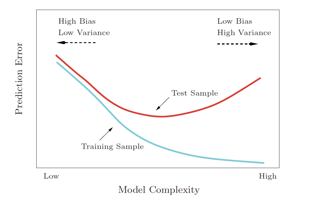
4 f_meas      binary         0.897

Bias-Variance Tradeoff

Test and training error as a function of model complexity. Note that the error goes down monotonically only for the training data. Be careful not to overfit!! image credit: ISLR

Reflecting on Model Building

Image credit: https://www.tmwr.org/

Reflecting on Model Building

Image credit: https://www.tmwr.org/

Reflecting on Model Building

Image credit: https://www.tmwr.org/

Support Vector Machines

Agenda 11/11/2024

`tidymodels` syntax

Support Vector Machines

Deriving SVM formulation

SVM applet

Agenda 11/13/24

What if the boundary is wiggly?

What if the boundary isn’t wiggly?

Examples of kernels

Big $C$ or small $C$ ?

Big $C$ or small $C$ ?

Big $C$ or small $C$ ?

Algorithm: Support Vector Machine

SVM example w defaults

Fit again

SVM example w CV tuning (RBF kernel)

SVM model output

SVM model output - take two

SVM model output - best CV parameters

SVM Final model – using CV params

SVM Final model – using `finalize_model()`

SVM Final model

Test predictions

Other measures

Bias-Variance Tradeoff

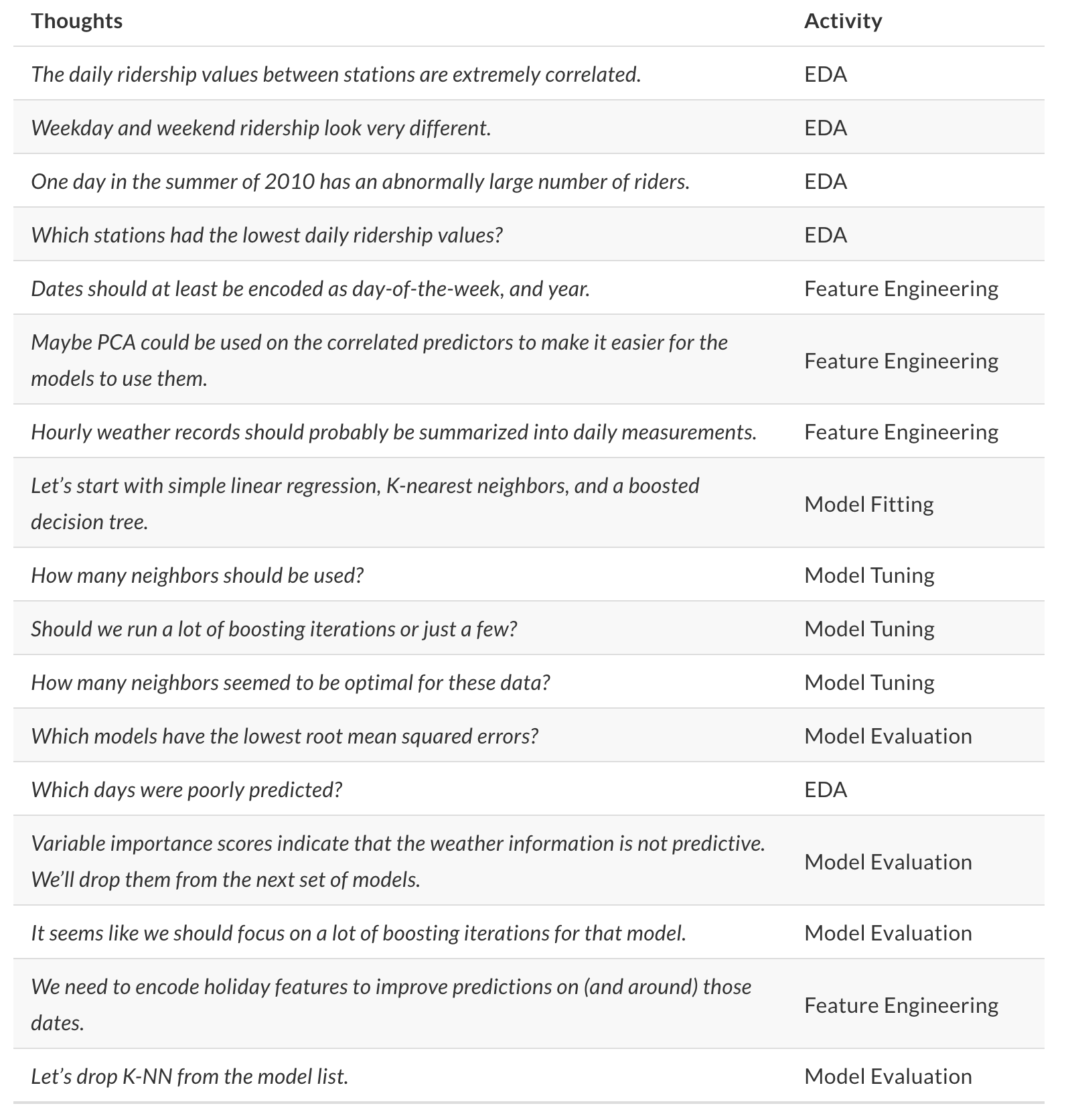
Reflecting on Model Building

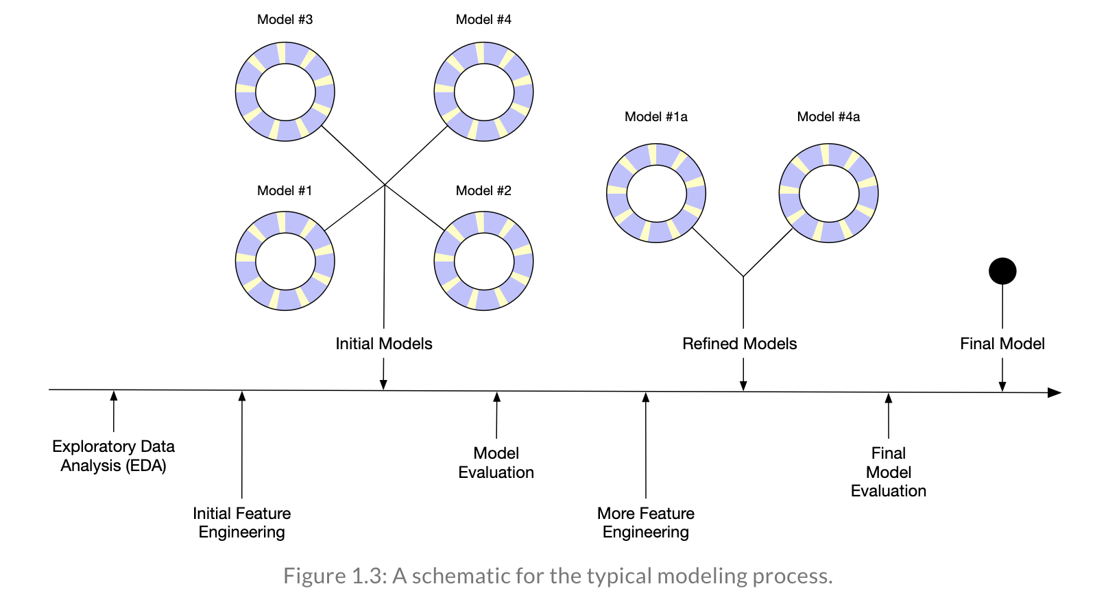
Reflecting on Model Building

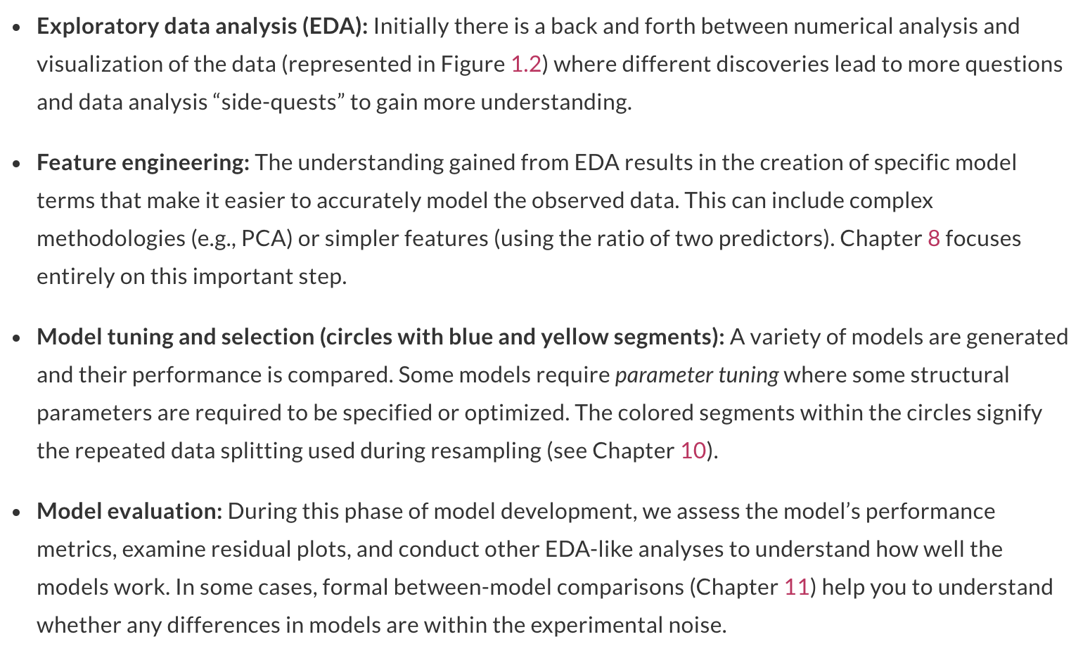
Reflecting on Model Building